Market-Orchestrated Protective Put

Following the framework introduced in the case of the covered call strategy, we now turn to its complementary component: the protective put. If the covered call represents a form of risk monetization through the sale of convexity, then the protective put represents a form of distribution insurance through the purchase of convexity¹.

Decision Framework: The Zone of Acceptance Link to heading

A protective put is not merely an insurance overlay — it is a deliberate redefinition of the acceptance region of outcomes.

Let $ S_T $ denote the terminal price of the underlying and $ K $ the strike of the put. The payoff structure becomes:

$$ \Pi_T = S_T + \max(K - S_T, 0) - P $$

where $ P $ is the premium paid.

The key observation is structural: the left tail is no longer open-ended — it is truncated at $ K - P $. We can therefore define the Zone of Acceptance as:

$$ \mathcal{A} = { \omega \mid \Pi_T(\omega) \geq L } $$

where $ L $ is a predefined loss threshold.

Unlike a naked long position, where $ \mathcal{A} $ is implicitly defined and often violated under stress scenarios, the protective put enforces a hard constraint on downside exposure.

This is not optimization — it is admissibility control. From an actuarial perspective, the strategy transforms the loss distribution from:

• heavy-tailed and unbounded on the left
  to
• bounded with a clearly defined worst-case outcome

This shift is critical when decisions are made under incomplete information: we are no longer required to estimate the extreme tail accurately — we eliminate its impact by construction.

Exit strategy Link to heading

The presence of the put fundamentally alters the logic of exit. In an unhedged position, exit decisions are typically reactive — driven by drawdowns, volatility spikes, or ex-post reassessment of expectations. This introduces path dependency and often leads to suboptimal timing.

Under a protective put, the exit becomes structurally pre-defined. There are only three coherent regimes:

• Downside breach ($ S_T \leq K $). The put is exercised (or monetized), and the position is exited at an effective level close to $ K - P $. No discretionary decision is required — the exit is automatic.

• Neutral zone ($ K < S_T \lesssim S_0 $). The underlying underperforms, but losses remain contained. The decision reduces to whether to:

  • roll the hedge (extend maturity), or
  • exit and reallocate capital. Importantly, this is a controlled decision space, not a forced liquidation.

• Upside realization ($ S_T \gg S_0 $). The hedge expires worthless, and the position behaves like a long asset minus premium. Exit becomes a question of opportunity cost rather than risk containment.²

The critical shift is this: the exit is no longer a response to uncertainty — it is embedded in the structure. This eliminates the most fragile component of investment behavior: decision-making under stress.

Structural Interpretation Link to heading

The protective put can be decomposed as:

$$ S_T + \max(K - S_T, 0) = \max(S_T, K) $$

so that:

$$ \Pi_T = \max(S_T, K) - P $$

This representation is not cosmetic — it reveals the true nature of the position:

• it is a long exposure with a floor
• equivalently, a synthetic guarantee on the terminal value

From a distributional standpoint, we replace a continuous payoff with one exhibiting a kink at $ K $, introducing convexity exactly where it is most valuable — in the loss region.

This has several non-trivial implications:

• Gamma profile becomes strongly positive near $ K $ → sensitivity increases precisely in stressed scenarios

• Vega exposure is positive → the position benefits from volatility expansion, which typically coincides with market distress

• Tail risk is no longer a modeling problem → it is a design choice already resolved at inception

However, a blind spot often ignored: the premium $ P $ is not a cost — it is the price of eliminating model dependence in the tail.

If volatility is overpriced, the strategy embeds a negative carry. If volatility is underpriced, it becomes a structural edge.

Market-Orchestrated Protective Put Link to heading

The protective put, as constructed above, presumes an existing long position in the underlying. But the position itself does not need to pre-exist — it can be induced, and the same mechanism used to induce it can, in the same motion, finance the hedge that protects it.

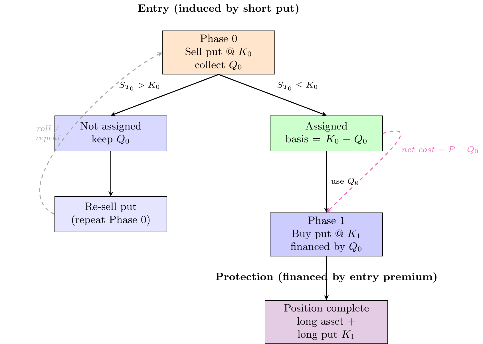
This is a multi-phase construction, not a simultaneous one. The sequencing matters.

Phase 0: Entry via a cash-secured short put

Let $ K_0 $ be the strike of a put written (sold) against cash collateral $ K_0 $ per contract, with premium $ Q_0 $ received at inception. This is the classical cash-secured put: a position that is only coherent when the investor already holds — and is willing to commit — the cash required to acquire the underlying at $ K_0 $.

Two terminal states exist at the expiry of this first put:

• Assignment ($ S_{T_0} \leq K_0 $). The underlying is acquired at $ K_0 $. The effective cost basis is: $$ B = K_0 - Q_0 $$ The long position — the very thing the protective put is meant to protect — now exists, and it was entered at a discount to $ K_0 $ by construction.

• Non-assignment ($ S_{T_0} > K_0 $). The put expires worthless. No position is entered; the investor retains $ Q_0 $ and the full collateral. Phase 0 can be re-initiated (rolled) at the next expiry, effectively being paid to wait for entry.

The key structural point:

Phase 0 is not a bet on direction — it is a conditional entry mechanism that is compensated (via $ Q_0 $) precisely in the branch where entry fails to occur, and that generates the financing for the hedge precisely in the branch where entry succeeds.

Phase 1: Financing the floor from $ Q_0 $

Upon assignment, the investor holds the underlying at basis $ B = K_0 - Q_0 $ and the premium $ Q_0 $ in hand. The protective put — strike $ K_1 $, premium $ P $ — is now purchased using some or all of $ Q_0 $ as its financing source.

The combined payoff, across both phases, collapses to:

$$ \Pi_T = S_T + \max(K_1 - S_T, 0) - B - P $$

$$ = S_T + \max(K_1 - S_T, 0) - K_0 + Q_0 - P $$

If $ Q_0 $ fully finances $ P $ (i.e. $ Q_0 = P $), the structure reduces to:

$$ \Pi_T = S_T + \max(K_1 - S_T, 0) - K_0 $$

a protective put whose premium cost has been entirely absorbed by the entry mechanism itself, at the price of accepting $ K_0 $ (not $ S_0 $) as the entry level.

If $ Q_0 > P $, the residual $ Q_0 - P $ is a net credit: the investor is paid to enter a fully-floored position. If $ Q_0 < P $, a residual debit remains, but one already reduced relative to an unfinanced protective put purchased directly at market entry.³

Why the Order of the Stages — Rather Than Simultaneity — Is Essential Link to heading

This construction is structurally different from a protection strategy applied to an existing position. The difference is not one of form, but of mechanism.

In the case of an existing position, protection is added subsequently. The investor already owns the asset and must find the resources required to purchase the protection. In the Phase 0 and Phase 1 construction, the sequence is reversed: the way in which the position is acquired generates the resource that will subsequently finance the protection.

More precisely, in Phase 0, the investor sells a put and receives the premium $ Q_0$. The underlying is actually acquired only if assignment occurs. At that point, the premium received can be used to purchase the protective put in Phase 1.

Therefore, the economic trade-off is not between the asset’s upside potential and protection against downside risk. Here, the trade-off is between entry price and downside protection.

The investor agrees to acquire the asset at $ K_0$, rather than purchase it at the market price $ S_0$, and is compensated for this willingness through the premium $ Q_0$. This premium can subsequently finance the protection provided by the purchased put.

In this construction, a market-orchestrated protective put does not, therefore, begin with buying a put. It begins with the willingness to own the asset at a predetermined price below the current market level and with turning that willingness into a source of financing for protection.

This makes Phase 0 a structural precondition, rather than merely an entry tactic. The construction is coherent only if the investor:

1. has sufficient cash to fully collateralize $ K_0$;
2. is genuinely willing to receive the underlying through assignment;
3. considers both outcomes of Phase 0 acceptable:
   • assignment, in which case the investor receives the underlying at an effective basis of $ B = K_0-Q_0$;
   • non-assignment, in which case the investor keeps the premium $ Q_0$ and fully recovers the collateral.

This last condition is essential. The investor must be genuinely indifferent between the two outcomes. If, in reality, the investor merely wants to collect the premium and hopes not to be assigned, then Phase 0 is no longer a coherent entry mechanism, but rather a disguised directional exposure.

Thus, the investor does not attempt to force entry into the market. The investor establishes in advance the conditions under which they are willing to enter, and the market determines whether those conditions are met.

This is precisely why sequencing matters. Phase 0 is not merely a stage that happens chronologically before Phase 1; it creates the economic condition for Phase 1. The premium $ Q_0$ is not generated by an already protected position, but by the process through which the position itself is induced.

In the absence of this indifference⁴, the construction reintroduces exactly the kind of reactive decision-making under stress that the protective put — once completed — was designed to eliminate.

Therefore, the structure does not attempt to predict the right moment to enter. It defines ex-ante the price we are willing to accept in order to become owners of the underlying and the protection we will purchase if that condition is induced. The rest is left to the market.

Conclusion Link to heading

The protective put can be viewed, in this construction, not merely as a protection instrument for an existing position, but as a complete decision structure in which both entry and exit can be determined entirely by market conditions.

At entry, the market determines whether the position is induced through assignment or whether the investor is paid to wait and repeat the mechanism. At exit, the same structural logic allows the protection threshold and exit conditions to be predefined through traded instruments, reducing the need for discretionary intervention precisely when such intervention is most vulnerable.

In this sense, the value of hedging lies not merely in reducing a potential loss. It lies in moving the decision from the investor’s mind into the structure of the market: entry conditions, risk acceptance, and exit limits are established ex-ante, and the market induces the mechanism when the predefined conditions are reached.

For an actuary, this is the difference between trying to predict every future realization and designing a structure in which an essential part of the decision is delegated to the market through predefined rules. We do not need to predict exactly what will happen; we only need to define in advance what we will do if certain conditions arise.

@online{Cornaciu2026ProtectivePut,
  author   = {Cornaciu, Valentin},
  orcid    = {0000-0001-9239-7145},
  title    = {Protective Put in Focus},
  year     = {2026},
  date     = {2026-08-16},
  url      = {https://rcor.ro/posts/2026-03-28-protective-put-in-focus/},
  abstract = {This article develops a structural interpretation of the protective put
  as a mechanism for redefining the acceptance region of investment outcomes. Rather 
  than treating hedging as an auxiliary overlay, the strategy is framed as an 
  admissibility constraint that truncates downside risk and embeds a pre-defined 
  exit rule. The analysis highlights the shift from reactive decision-making to
  structurally enforced outcomes, emphasizing the role of convexity, volatility 
  exposure, and tail-risk elimination. Particular attention is given to the premium
  as the price of reducing model dependence in the tail, thereby positioning the 
  protective put as a statement about uncertainty rather than a simple 
  risk mitigation tool.}
}

This is the cornerstone of market investing, anchoring strategies in statistical inference, and grounded in disciplined risk management and actuarial principles. It is not necessary to master every detail of the underlying models—what matters is the ability to identify a qualified actuary who can construct and validate the appropriate framework, ensuring consistency, robustness, and alignment with the underlying risk structure.