Beyond Empirical Correlation: A Structural VIX Decomposition Approach

Financial markets often exhibit a strong negative correlation between equity prices and the VIX index. While this relationship is usually measured empirically from historical observations, the construction of VIX itself suggests a different approach.

The VIX is not an arbitrary market indicator. It is explicitly defined as a weighted portfolio of out-of-the-money SPX options. Consequently, before attempting to estimate

$$ \mathrm{cor}(X,\mathrm{VIX}), $$

for some stock X, it is natural to first understand how VIX itself decomposes into option prices.

The CBOE VIX Formula Link to heading

The VIX methodology published by the CBOE defines the risk-neutral expected variance over a future horizon $ T$ as

$$ \sigma^2(T) = \frac{2e^{RT}}{T} \sum_i \frac{\Delta K_i}{K_i^2} Q(K_i) - \frac{1}{T} \left( \frac{F}{K_0} - 1 \right)^2\tag{1} $$

where:

• $ T$ is the time to expiration (in years). In the VIX calculation, Equation (1) is evaluated twice: once for the near-term expiration $ T_1$ and once for the next-term expiration $ T_2$¹
• $ R$ is the risk-free interest rate to expiration;²
• $ F=K + e^{RT}\bigl(C(K)-P(K)\bigr)$ is the option-implied forward index level, where $ K$ is the strike for which the absolute difference between call and put prices is smallest;
• $ K_0$ is the first strike equal to or otherwise immediately below the forward index level, $ F$;³
• $ \Delta K_i = \frac{K_{i+1}-K_{i-1}}{2}$ is the interval between strike prices (half the difference between the strikes on either side of $ K_i$);
• $ Q(K_i)$ is the midpoint of the bid-ask spread for each option with strike $ K_i$.

$$ Q(K)= \begin{cases} P(K), & K < K_0,\\ \dfrac{P(K)+C(K)}{2}, & K = K_0,\\ C(K), & K > K_0. \end{cases}$$

The final VIX value is obtained by calculating the 30-day weighted average of $ \sigma^2_1$ and $ \sigma^2_2$, taking the square root of that value, and multiplying by 100:

$$ \text{VIX} = 100 \times \sqrt{ \left[ T_1 \sigma^2_1 \left( \frac{N_{T_2} - N_{30}}{N_{T_2} - N_{T_1}} \right) + T_2 \sigma^2_2 \left( \frac{N_{30} - N_{T_1}}{N_{T_2} - N_{T_1}} \right) \right] \times \frac{N_{365}}{N_{30}} } $$

Therefore VIX is built from a strip of out-of-the-money puts and calls spanning a large range of strikes.

VIX as a Portfolio of Options Link to heading

Ignoring for the moment the small forward-adjustment term,

$$ \frac{1}{T} \left( \frac{F}{K_0} -1 \right)^2, $$

the variance estimate can be written as

$$ \sigma^2(T) \approx \sum_i w_i Q(K_i), $$

with weights

$$ w_i=\frac{2e^{RT}}{T}\frac{\Delta K_i}{K_i^2}. $$

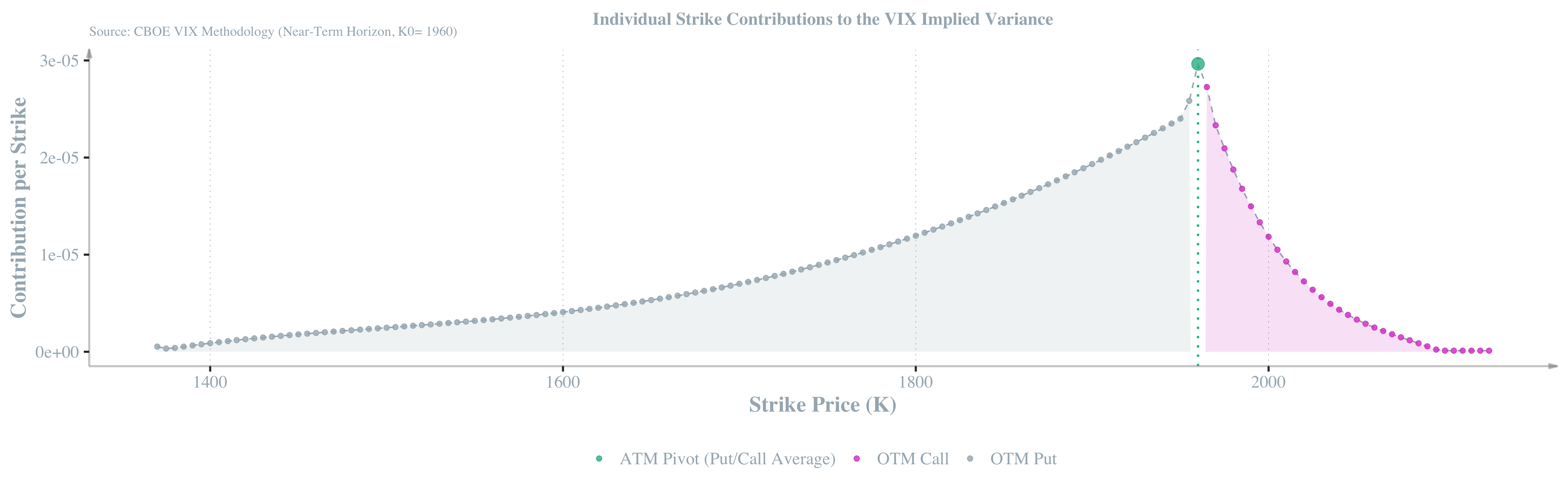
This representation immediately reveals a key property of VIX. Every option contributes positively, but the contribution is inversely proportional to $ K_i^2$. Lower strikes therefore receive significantly larger weights than higher strikes. Although the summation extends over a wide range of strikes, option prices for sufficiently deep out-of-the-money (OTM) contracts rapidly approach zero, so their contribution to the variance estimate becomes negligible.

The decomposition implies a structural asymmetry: strikes below $ K_0$ enter exclusively through OTM puts, while strikes above $ K_0$ enter through OTM calls. Since downside options embed stronger convexity under the risk-neutral measure, the resulting variance estimate is more sensitive to changes in put prices than to comparable changes in call prices. This is conceptually closer to the asymmetry in a covered-call-type exposure, where upside and downside risks are not treated symmetrically.

Reconstructing the Underlying from Options Link to heading

Once VIX has been expressed entirely through option prices, it becomes natural to ask whether the underlying asset itself can be represented similarly. The answer is yes.

Put-call parity states that

$$ C(K)-P(K)=e^{-RT}(F-K) $$

Rearranging,

$$ F=K+e^{RT}\bigl(C(K)-P(K)\bigr). $$

Since the spot price satisfies

$$ S_0=e^{-RT}F, $$

we obtain

$$ S_0=e^{-RT}K+C(K)-P(K). $$

For every strike $ K$, the stock can therefore be replicated by a bond position together with a long call and a short put.

A Strike-by-Strike Decomposition Link to heading

Repeating the parity relation across many strikes gives

$$ S_0=\sum_i\alpha_i\left[e^{-RT}K_i+C(K_i)-P(K_i)\right], $$

for any set of weights satisfying

$$ \sum_i \alpha_i = 1. $$

This representation places the stock and the VIX on a common footing:

• VIX is a weighted combination of option prices;
• the stock can also be represented through option prices using put-call parity.

Towards a Correlation Decomposition Link to heading

The traditional estimate of

$$ \mathrm{cor}(X,\mathrm{VIX}) $$

uses historical observations of $ X$ and VIX.

However, after expressing both quantities through option prices, the correlation can be viewed as emerging from the dependence structure between

$$ P_X(K), \qquad C_X(K), \qquad P_{SPX}(K), \qquad C_{SPX}(K). $$

Rather than correlating two observed time series, one may attempt to correlate their option-based decompositions.

This perspective suggests a new path toward understanding why different stocks exhibit different sensitivities to market volatility and tail-risk pricing.

Implication for dependence with an underlying variable X Link to heading

Since the market is incomplete, one should not expect a unique representation of the dependence between X and the VIX. Instead, the analysis should consider the set of feasible transformations, namely those that can be constructed from observable market data and are consistent with the market’s constraints and trading mechanisms.

When studying dependence between an underlying variable $ X$ and VIX, a direct Pearson or Spearman correlation is generally misaligned with the construction above. The transformation from option prices to VIX introduces

• strong nonlinearity (square-root of a weighted integral),
• asymmetric sensitivity (left-tail dominated weighting),
• aggregation across two maturities ($ T_1$ and $ T_2$),
• and a projection from a high-dimensional object (the option surface) to a scalar.

Therefore, a more meaningful object of study is

$$ \mathrm{cor}\bigl(g(X), h(\mathrm{VIX})\bigr), $$

where $ g$ and $ h$ are transformations chosen to align the variables with the structural sensitivities embedded in the VIX construction.

The transformation $ g$ may emphasize features of the underlying that are economically related to implied variance, while $ h$ determines whether the analysis concerns the level of implied volatility or volatility shocks.

Examples of operationally meaningful transformations include:

• for $ g$: log-returns, realized variance, absolute returns, downside returns, or tail-event indicators;
• for $ h$: VIX levels, first differences, simple returns, or logarithmic returns.

Using logarithmic returns for both variables measures the association between daily shocks. In contrast, using the realized standard deviation for X together with the VIX level compares ex-post realized volatility over a given time interval with the market’s ex-ante⁴ expectation of future volatility.

The objective is not to maximize correlation in a purely statistical sense, but to construct a dependence measure that is consistent with the pricing functional underlying VIX.

An additional implication concerns the time horizon over which correlation is estimated.

Since VIX reflects the market price of approximately 30-day forward variance rather than a persistent economic characteristic, its dependence on an underlying variable is itself regime dependent. Monetary policy, market structure, liquidity, and investors’ demand for downside protection evolve through time, altering this relationship.

Consequently, estimating a single correlation over a decade or longer implicitly assumes that the dependence remains stable throughout the sample, an assumption with little economic justification.

A more meaningful approach is to estimate the dependence over relatively short horizons, such as rolling windows of approximately one year. This allows both the transformations $ g$ and $ h$, and the resulting dependence measure, to reflect the prevailing market regime rather than averaging across fundamentally different environments.

Conclusion Link to heading

The CBOE methodology shows that VIX is fundamentally a weighted portfolio of out-of-the-money options. Using put-call parity, a stock can likewise be represented through option positions.

Expressing both quantities in terms of options creates a common mathematical framework and opens the possibility of studying correlations directly at the level of option prices rather than only through historical returns.

Whether such a decomposition leads to more stable or more informative estimates of correlation remains an open question, but it provides a natural starting point for further investigation.

This is the cornerstone of market investing, anchoring strategies in statistical inference, and grounded in disciplined risk management and actuarial principles. It is not necessary to master every detail of the underlying models—what matters is the ability to identify a qualified actuary who can construct and validate the appropriate framework, ensuring consistency, robustness, and alignment with the underlying risk structure.

@online{Cornaciu2026VIX,
  author   = {Cornaciu, Valentin},
  orcid    = {0000-0001-9239-7145},
  title    = {Beyond Empirical Correlation: A Structural VIX Decomposition Approach},
  year     = {2026},
  date     = {2026-07-10},
  url      = {https://rcor.ro/posts/2026-06-16-beyond-empirical-correlation-a-structural-vix-decomposition-approach},
  abstract = {This article interprets the VIX through the CBOE methodology,
  showing that it is fundamentally a weighted portfolio of out-of-the-money
  options. Using put-call parity, the underlying asset is expressed within the
  same mathematical framework, making it possible to formulate a decomposition
  of correlation directly in terms of option prices. The paper further discusses
  suitable transformations of the underlying variable and VIX, together with the
  limitations of estimating correlations over excessively long historical horizons.}
}