Two Heads in a Row — Success Is Pinker Than It Seems

We flip a fair coin repeatedly and stop as soon as we observe two heads in a row HH. What is the expected number of flips?

When flipping a fair coin until observing two consecutive heads (HH), a common initial intuition suggests an expected waiting time related to $ p = 1/4$ (i.e., 4 flips¹). However, this naive calculation assumes independent blocks of size two, ignoring the sliding-window nature and the asymmetric failure resets inherent in sequence matching.

To model this process, we use a simple application of Bellman’s Principle of Optimality. This is a particularly straightforward case: there is only one available action — flipping the coin — and every action has the same immediate cost of 1 flip. The only source of uncertainty is the outcome of the coin toss, which determines the next state.

This allows us to express the expected remaining cost recursively, transforming an infinite-horizon problem into a finite system of equations. For a more general discussion of Bellman’s Principle of Optimality Bellman (1952), including the conditions under which it applies, see Choosing the Right Path.

Bellman’s Principle of Optimality Link to heading

Under Dynamic Programming, the value function $ V(s)$ represents the expected number of additional flips needed to reach the target sequence, starting from state $ s$. We define the state space based on the current streak of consecutive heads:

• $ S_0$: Baseline state (no previous head OR last flip was Tails).
• $ S_1$: Partial progress state (last flip was Heads).
• $ S_2$: Terminal state (HH achieved, $ V(S_2) = 0$).

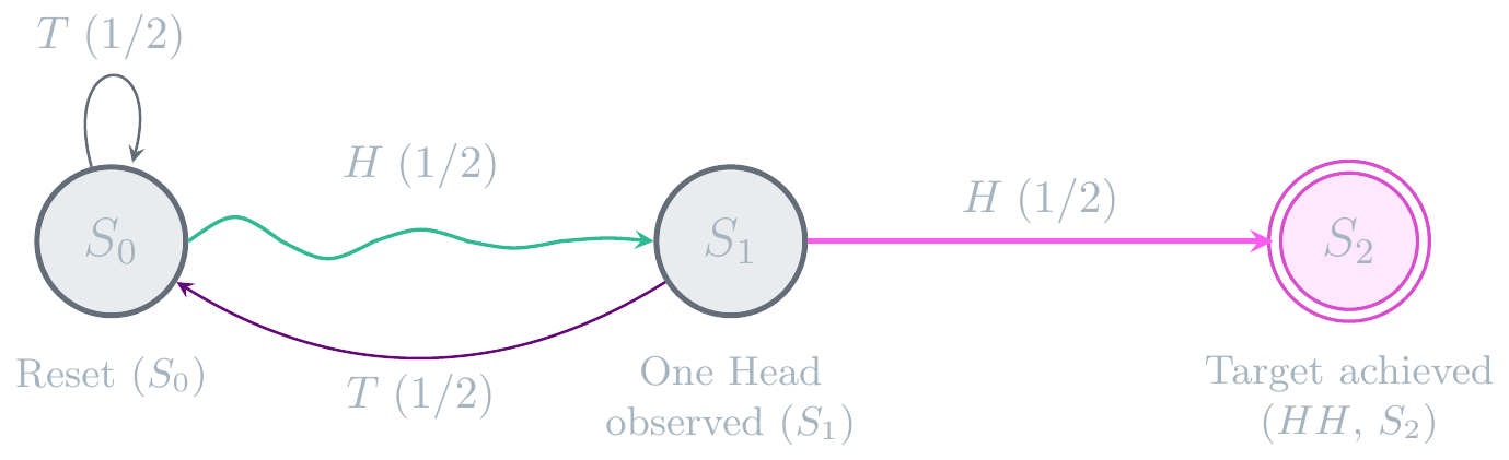
Under the Bellman Expectation Equation, the value function $ V(S)$—representing the remaining expected number of flips from state $ S$—satisfies:

V(S) = 1 + \mathbb{E}\big[ V(S') \mid S \to S' \big] \tag{1}

The first term $ 1$, represents the cost of performing the next flip. The conditional expectation expands directly over the state space transitions. For the baseline state $ S_0$, this expectation becomes:

\mathbb{E}\big[V(S') \mid S_0 \to S' \big] = V(S_0)\cdot p(S_0 \mid S_0) + V(S_1) \cdot p(S_1 \mid S_0) \tag{2}

Substituting the conditional expectations into the Bellman equation gives the following system:

\begin{cases}
V(S_1) = 1 + \frac{1}{2} V(S_0) + \frac{1}{2}\underbrace{V(S_2)}_{0}, \\\
V(S_0) = 1 + \frac{1}{2} V(S_0) + \frac{1}{2} V(S_1)
\end{cases} \tag{3}

Solving this 2-state system yields concrete values for $ V(S_0)=6$ and $ V(S_1)=4$. However, as the state space expands to $ n$ ssequential milestones or risk checkpoints, solving linear systems manually becomes intractable. To evaluate arbitrary processes with $ n$ distinct states and varying success probabilities $ p_k$, we must scale this recurrence relationship into a closed-form analytical solution.

Deriving the General Formula Link to heading

Let $ V_k $ denote the expected number of additional steps needed to reach the target state $ S_n $, starting from state $ S_k $.

At each state $ S_k $, for $ k {0, 1, , n-1} $, the process has two possible transitions:

• Advance to state $ S_{k+1} $ with probability $ p_k $.
• Reset to the initial state $ S_0 $ with probability $ 1-p_k $.

Assuming that $ 0 < p_k $, the Bellman equation for state $ S_k $ is:

V_k = 1 + p_k V_{k+1} + (1-p_k)V_0  

The term $ 1 $ accounts for the step just taken, while the remaining terms represent the expected number of additional steps after the transition. The boundary condition is $ V_n = 0$ since no additional steps are needed once the target state has been reached. We can derive $ V_0 $ by successively substituting the Bellman equations.

1. Starting from state $ S_0 $:

V_0 = 1 + p_0 V_1 + (1-p_0)V_0

Rearranging gives:

V_1 = V_0 - \frac{1}{p_0}

2. Starting from state $ S_1 $:

V_1 = 1 + p_1 V_2 + (1-p_1)V_0

Substituting the expression for $ V_1 $:

V_0 - \frac{1}{p_0} = 1 + p_1 V_2 + (1-p_1)V_0

Rearranging:

V_0 = \frac{1}{p_1} + \frac{1}{p_0 p_1} + V_2

3. Continuing by substitution:

Each successive substitution introduces another reciprocal transition probability. After $ n $ substitutions, we obtain:

V_0 = \frac{1}{p_0} + \frac{1}{p_0p_1} + \cdots + \frac{1}{p_0p_1\cdots p_{n-1}} + V_n

Using the boundary condition $ V_n = 0 $, the general formula follows:

V_0 = \sum_{k=0}^{n-1} \prod_{j=0}^{k} \frac{1}{p_j}

Thus, the expected number of steps to reach the target is the sum of the reciprocals of the probabilities of successfully completing each successive sequence of transitions.

This result applies to reset-to-zero processes in which each unsuccessful transition returns the process to $ S_0 $, while each successful transition advances it by exactly one state.

Derivation of the exact distribution Link to heading

Let $ N$ be the random variable representing the total number of flips needed to observe two consecutive heads (HH) for the first time. Let $ a_k$ be the number of valid sequences of length $ k$ that end in HH for the first time.

For $ k \ge 2$:

• $ k = 2$: HH $ \implies a_2 = 1$.
• $ k = 3$: THH $ \implies a_3 = 1$.
• For $ k \ge 4$, a valid sequence of length $ k$ ending in HH for the first time must either:

1. Start with T followed by a valid sequence of length $ k-1$ $ \implies a_{k-1}$
2. Start with HT² followed by a valid sequence of length $ k-2$ $ \implies a_{k-2}$

Thus, the number of successful outcomes obeys the Fibonacci-like recurrence relation:

a_k = a_{k-1} + a_{k-2}, \quad \text{for } k \ge 4, \quad \text{with } a_2 = 1, a_3 = 1.

Since every sequence of length $ k$ has $ 2^k$ equally likely outcomes, the exact Probability Mass Function (PMF) is:

P(N = k) = \frac{a_k}{2^k} = \frac{F_{k-1}}{2^k}, \quad \text{for } k \ge 2

where $ F_m$ is the m-th Fibonacci number ($ F_1 = 1, F_2 = 1, F_3 = 2, F_4 = 3, \dots$).

In , we can approximate the sequence using:

RV(2:1000,sapply(2:1000, function(k) numbers::fibonacci(k-1)/2^k),fractions=F,remove=F)⏎ 
════════════════════════════════════════════════════════════════════════════════════════
Random variable with |999⟩ events, (µ = 6 | σ = 4.69), entropy 2.49
──
ᴿᵢ      2      3      4      5      6      7      8      9     10     11     12     13     14     15     16     17     18     19     20     21     22     23     24     25     26     27     28     29     30     31     32
ᵖᵢ 0.2500 0.1250 0.1250 0.0938 0.0781 0.0625 0.0508 0.0410 0.0332 0.0269 0.0217 0.0176 0.0142 0.0115 0.0093 0.0075 0.0061 0.0049 0.0040 0.0032 0.0026 0.0021 0.0017 0.0014 0.0011 0.0009 0.0007 0.0006 0.0005 0.0004 0.0003
ℹ Displaying the first 31 significant values* with extremes [2:78], VaR(99.5%) = 26.

The Reset Paradox Link to heading

In Fundamentals: Ten Keys to Reality, Nobel laureate Frank Wilczek Wilczek (2021) proposes an extraordinarily simple algorithm for producing the complete works of Shakespeare:

• Choose an ASCII character – a letter, number, space, or punctuation mark – at random.
• record it,
• repeat

This is also known as the Monkey Shakespeare³ thought experiment: a monkey randomly types characters from an alphabet, hoping to reproduce a predetermined sequence of $ n $ characters. Assume an alphabet of $ m $ equally likely symbols and a strict-reset mechanism: every incorrect character erases all accumulated progress, returning the process to its initial state $ S_0 $.

At each position, the probability of typing the required character is $ p_k = 1/m $. Substituting this into our general Bellman solution gives:

V_0 = \sum_{k=0}^{n-1} m^{k+1} = m \left( \frac{m^n - 1}{m - 1} \right) = \frac{m}{m-1}m^n - \frac{m}{m-1}

A striking mathematical property emerges. For an alphabet of 27 characters ($ m = 27 $), the multiplicative factor approaches: $ \frac{m}{m-1} = \frac{27}{26} \approx 1.03846$

The paradox: Intuitively, a strict-reset mechanism seems extremely inefficient. A single incorrect character wipes out all accumulated progress, forcing the process to start again from scratch. One might expect these repeated failures to introduce substantial additional waiting time.

Yet the closed-form solution tells a different story. Relative to the baseline scale $ m^n $, the expected waiting time approaches a factor of just $ 1.03846 $⁴. In other words, the reset mechanism adds only about 3.85% overhead, even as the target sequence grows from 20 to 200 characters.

More precisely, the relative overhead is:

\frac{V_0}{m^n} - 1 = \frac{1-m^{1-n}}{m-1}

As $ n $, the term $ m^{1-n} $ vanishes, and the overhead converges to:

\lim_{n\to\infty}\left(\frac{V_0}{m^n}-1\right) = \frac{1}{m-1} = \frac{1}{26} \approx 3.85\%

The result is counterintuitive: even though every failure destroys all accumulated progress, the expected cost of these resets remains remarkably small relative to the exponentially growing baseline.

However, the expected value does not tell the whole story. If we require a 99.5% probability of success, we need to consider the upper tail of the waiting-time distribution. For large $ n $, the waiting time is approximately exponentially distributed. Its 99.5% quantile is therefore⁵:

Q_{99.5\%} \approx -\ln(0.005)·V_0 \approx 5.2983·V_0

Combining this with the expected waiting time gives:

Q_{99.5\%} \approx 5.5021·27^n

In other words, while the expected waiting time is only about 3.85% above the baseline, achieving a 99.5% probability of success requires approximately 5.5 times the baseline.

A comparison Link to heading

We can apply the same reasoning to several random experiments. We report bellow both the expected waiting time and the 99.5% quantile (SCR).

Conclusion Link to heading

The probability of reproducing the entire sequence on the first attempt is more than just a measure of the initial difficulty. In a model with independent attempts and a strict reset mechanism, its reciprocal provides a natural benchmark for the expected waiting time.

Paradoxically, the difference between this benchmark and the actual expected waiting time depends on the structure of the experiment. In the case of HH, overlapping attempts increase the expected waiting time from 4 to 6 flips — a 50% increase. The Monkey Shakespeare model, however, leads to a seemingly opposite result. With a strict reset mechanism and an alphabet of 27 characters, the actual expected waiting time exceeds the benchmark by less than 3.85%, regardless of the target sequence’s length.

The key distinction lies in the structure of the process: the effect of repeated attempts is not determined by the probability of success on the first attempt alone, but also by how the experiment handles partial progress and failure.

What seems impossible to achieve on the first attempt may not be so far out of reach after all.⁷ Even when the target is an entire work, failing on the first attempt adds surprisingly little to the overall expected waiting time. The first step does not have to be perfect⁸; what matters is understanding the cumulative cost of starting over until we succeed.

Moreover, the mean is not sufficient to characterize risk. The 99.5% quantile shows how far the waiting time can exceed its expected value, offering a different perspective that is essential for capital adequacy and the assessment of extreme risk.

This way of thinking defines the core of Actuarial Mathematics, particularly as illustrated by credibility theory. You don’t need to know everything. You need to know what to ask, what initial conditions to start from, what to verify, and whom to entrust with the problem.

The author declares no competing financial interests or personal relationships that could have influenced the work presented in this article.

@online{Cornaciu2026HH,
  author   = {Cornaciu, Valentin},
  orcid    = {0000-0001-9239-7145},
  title    = {Two Heads in a Row},
  year     = {2026},
  date     = {2026-11-10},
  url      = {http://rcor.ro/posts/2026-10-31-two-heads-in-a-row/},
  abstract = {This article examines the problem of repeatedly tossing a fair coin until
  two consecutive heads appear. Using Bellman's principle of optimality, it derives the
  expected waiting time through a state-transition model and explores the full waiting-
  time distribution. The analysis connects dynamic programming, recurrence relations, 
  and Fibonacci numbers, illustrating how the same process can be understood from both
  an expectation-based and a distributional perspective. It also examines the reset 
  mechanism in the Monkey Shakespeare experiment, showing that repeated failures can 
  add only a small relative overhead to the expected waiting time. The distinction 
  between expected performance and tail risk highlights the importance of choosing the
  right measure when evaluating stochastic processes.}
}